Sift : Scale Space

01 September 2013

DoG尺度空间生产

GSS(Gauss Scale-space)

It has been shown by Koenderink (1984) and Lindeberg (1994) that under a variety of reasonable assumptions the only possible scale-space kernel is the Gaussian function. Therefore, the scale space of an image is deﬁned as a function, $L(x,y,\sigma)$, that is produced from the convolution of a variable-scale Gaussian, $G(x,y,\sigma)$ , with an input image, $I(x, y)$ :

唯一能产生尺度空间的核为高斯核函数，所以我们将图像的尺度空间表示成一个函数 $L(x,y,\sigma)$，它是由一个变尺度的高斯函数 $G(x,y,\sigma)$ 与图像 $I(x, y)$ 卷积产生的。即

$$ L(x,y,\sigma)=G(x, y, \sigma) \ast I(x, y) $$

其中 $\ast$ 代表卷积操作，$G(x, y, \sigma)$ 为二维高斯核函数，表示为：

$$ G(x, y, \sigma) =\frac{1}{2\pi\sigma^{2}}e^{-(x^{2}+y^{2})/2\sigma^{2}} $$

DoG(Difference of Gauss)　　

DoG生成

SIFT算法建议，在某一尺度上对特征点的检测，可以通过对两个相邻高斯尺度空间的图像相减，得到一个 DoG (Difference of Gaussians)的响应值图像 $D(x,y,\sigma)$ 。然后，仿照 LoG 方法，通过对响应值图像 $D(x,y,\sigma)$ 进行非最大值抑制(局部极大搜索，正最大和负最大)，在位置空间和尺度空间中定位特征点。其中

$$D(x, y, \sigma) = \left [ G(x, y, k\sigma) − G(x, y, \sigma) \right ] \ast I(x, y) = L(x, y, k\sigma) − L(x, y, \sigma)$$

式中，$k$ 为相邻尺度空间倍数的常数。

为什么用DoG来检测特征点

In addition, the difference-of-Gaussian function provides a close approximation to the scale-normalized Laplacian of Gaussian, $\sigma^{2}\nabla^{2}G$, as studied by Lindeberg (1994). Lindeberg showed that the normalization of the Laplacian with the factor $\sigma^{2}$ is required for true scale invariance. In detailed experimental comparisons, Mikolajczyk (2002) found that the maxima and minima of $\sigma^{2}\nabla^{2}G$ produce the most stable image features compared to a range of other possible image functions, such as the gradient, Hessian, or Harris corner function.

Lindeberg证明用 $\sigma^{2}$ 标准化的高斯拉普拉斯($\nabla^{2}G$, LOG, Laplacian of Gauss)有着真正的尺度无关的特性，而 Mikolajczyk 发现，相比于其他一系列函数（比如梯度，Hessian，Harris角点函数等），用$\sigma^{2}$标准化的高斯拉普拉斯($\sigma^{2}\nabla^{2}G$)有着更稳定的图像特征，因此 $\sigma^{2}\nabla^{2}G$ 函数是我们理想的寻找特征点的函数。而在此，我们利用 DoG 来近似 $\sigma^{2}\nabla^{2}G$。

通过热传导方程也可以帮助我们理解 DoG 与 $\sigma^{2}\nabla^{2}G$ 之间的近似关系。由热传导方程可知（通常用 $t = \sigma^{2}$）:

$$\frac{\partial G}{\partial \sigma}=\sigma\nabla^{2}G$$

对上式进行有限差分运算得：

$$\sigma\nabla^{2}G=\frac{\partial G}{\partial \sigma}\approx =\frac{G(x,y,k\sigma)-G(x,y,\sigma)}{k\sigma-\sigma}$$

因此

$$DoG=G(x,y,k\sigma)-G(x,y,\sigma)\approx (k-1)\sigma^{2}\nabla^{2}G$$

而常数项$(k - 1)$并不会影响极值的位置。所以 DoG 是 $\sigma^{2}\nabla^{2}G$ 的近似。

对于使用 DoG 来近似 $\sigma^{2}\nabla^{2}G$，有如下优点：

$\sigma^{2}\nabla^{2}G$ 需要使用两个方向的高斯二阶微分卷积核，而 DoG 直接使用高斯卷积核，省去了对卷积核的生成的运算量。
DoG 保留了各个高斯尺度空间的图像，这样，在生成某一空间尺度的特征时，可以直接尺度空间图像，而无需重新再次生成该尺度的图像。

GSS尺度选择

GSS中尺度值的产生

由上一节知 DoG 近似于 $(k − 1)\sigma^{2}\nabla^{2}G$，对于常数 $k$，即为相邻高斯尺度空间的两幅图像的尺度倍数，Lowe在文中提到

The approximation error will go to zero as k goes to 1, but in practice we have found that the approximation has almost no impact on the stability of extrema detection or localization for even signiﬁcant differences in scale, such as $k = \sqrt{2}$.

文中提到k值大小对于极值的检测没有什么影响。那么 $k$ 究竟取多大呢？　　

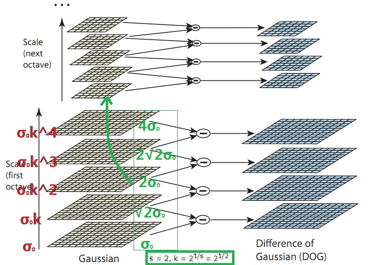
We choose to divide each octave of scale space (i.e., doubling of $\sigma$) into an integer number, $s$, of intervals, so $k = 21/s$. We must produce $s + 3$ images in the stack of blurred images for each octave, so that ﬁnal extrema detection covers a complete octave. Adjacent image scales are subtracted to produce the difference-of-Gaussian images shown on the right. Once a complete octave has been processed, we resample the Gaussian image that has twice the initial value of $\sigma$ (it will be 2 images from the top of the stack) by taking every second pixel in each row and column. The accuracy of sampling relative to σ is no different than for the start of the previous octave, while computation is greatly reduced.

问题1 为什么用前一个octave中的倒数第三幅图像生成下一octave中的第一幅图像？

我们通过上图来解释这段话，由 “must produce $s + 3$ images in the stack of blurred images for each octave” 可知每层octave产生了5幅图像，所以 $s = 2$。同一 octave 相邻图像之间尺度为 $k$ 倍的关系， $k = 2^{1/s} = 2^{1/2}$，仔细阅读上一段下划线部分，当完成一层 octave 的处理后，对2倍 $\sigma$ 的高斯图像（即用尺度大小为 $2\sigma$的高斯函数模糊的图像）进行二分重采样，得到下一个 octave 的第一幅图像。而这个用尺度大小为 $2\sigma$ 的高斯函数模糊的图像总是处于该 octave 的倒数第三幅（由上往下数，第三幅。原文：it will be 2 images from the top of the stack，程序员都是从0开始数的咯），因为总共一层 octave 为 $s+3$ 幅图像，第 $n$ 层即为 $k^{n}\sigma_{0}$(其中 $n = 0,1,\cdots,s,s+1,s+2$, $k = 2^{1/s}$)，当 $n$ 等于 $s$ 时，$k^{n}σ_{0} = 2σ_{0}$，第 $s$ 层即为倒数第三层。

Drawing

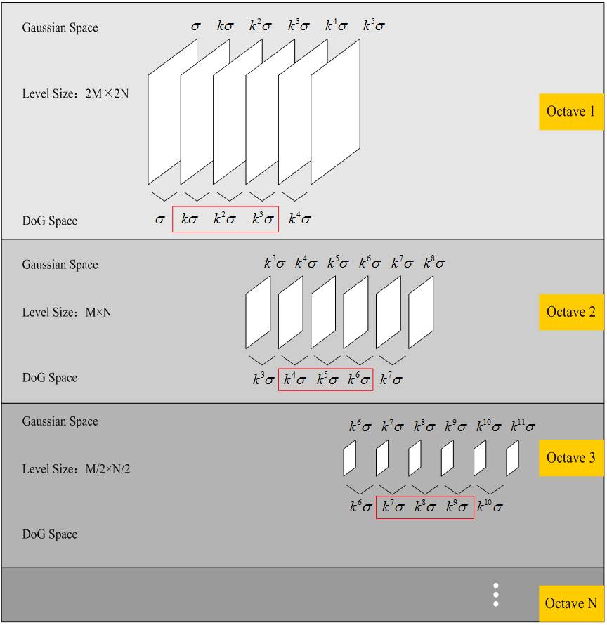
问题2 每层octave为什么生成 $s+3$ 幅图像？

在极值比较的过程中，每一组图像的首末两层是无法进行极值比较的，为了满足尺度变化的连续性，生成高斯金字塔每组有 $s+3$ 层图像。DOG金字塔每组有 $s+2$ 层图像。见上图，为 $s = 3$ 的情况，由上一问题可知，GSS 中倒数第三幅尺度与下一 octave 第一幅的尺度相同，由图中红色矩形中的尺度对应为 DoG 中极值检测的图像，将其各层红色矩形框中的尺度依次排列，即可发现其为以 $k = 2^{1/s}$（即 $k = 2^{1/3}$）为等比的连续尺度。所以极值检测是在一个连续变化的尺度空间中进行的。如下图：

Drawing

高斯核性质及其在SIFT中的应用

对于二维高斯卷积，有如下性质：

距离高斯核中心 $3\sigma$ 距离外的系数很小，相对于 $3\sigma$ 内的系数值可以忽略不计，所以只用 $(6\sigma + 1)\times(6\sigma + 1)$ 的面积计算卷积即可。
线性可分，二维高斯核卷积（计算次数 $O(n^{2}\cdot M\cdot N)$）效果等于水平和竖直方向的两个一维高斯核（计算次数 $O(n\cdot M\cdot N)+O(n\cdot M\cdot N)$）累积处理的效果。$n\cdot n$ 为滤波器大小，$M\cdot N$ 图像大小
对一幅图像进行多次连续高斯模糊的效果与一次更大的高斯模糊可以产生同样的效果，大的高斯模糊的半径是所用多个高斯模糊半径平方和的平方根。例如，使用半径分别为 6 和 8 的两次高斯模糊变换得到的效果等同于一次半径为 10 （勾股定理）的高斯模糊效果。根据这个关系，使用多个连续较小的高斯模糊处理不会比单个高斯较大处理时间要少。

其中，性质3有助我们更快速的生成GSS。虽然两个小半径处理时间并不会比单个高斯较大半径处理的时间少，但相对于原图像，我们已经有一个小半径模糊过的图像，即可用另一小半径在现成的图像上进行模糊得到较大半径的模糊效果。例如尺度为 $\sigma_{0}$ 的图像已经存在，我们要得到尺度为 $k\sigma_{0}$ 的图像，即可只使用尺度为 $((k\sigma_{0})^{2}-(\sigma_{0})^{2})^{1/2}$ 的核在尺度为 $\sigma_{0}$ 的图像上进行模糊，即可得到尺度为 $k\sigma_{0}$ 模糊的图像，同理可得到高斯尺度空间各层的图像，使得高斯尺度空间生产得更快。

参考资料：